Wavetable Studies
Iterative Indices (f+n2)
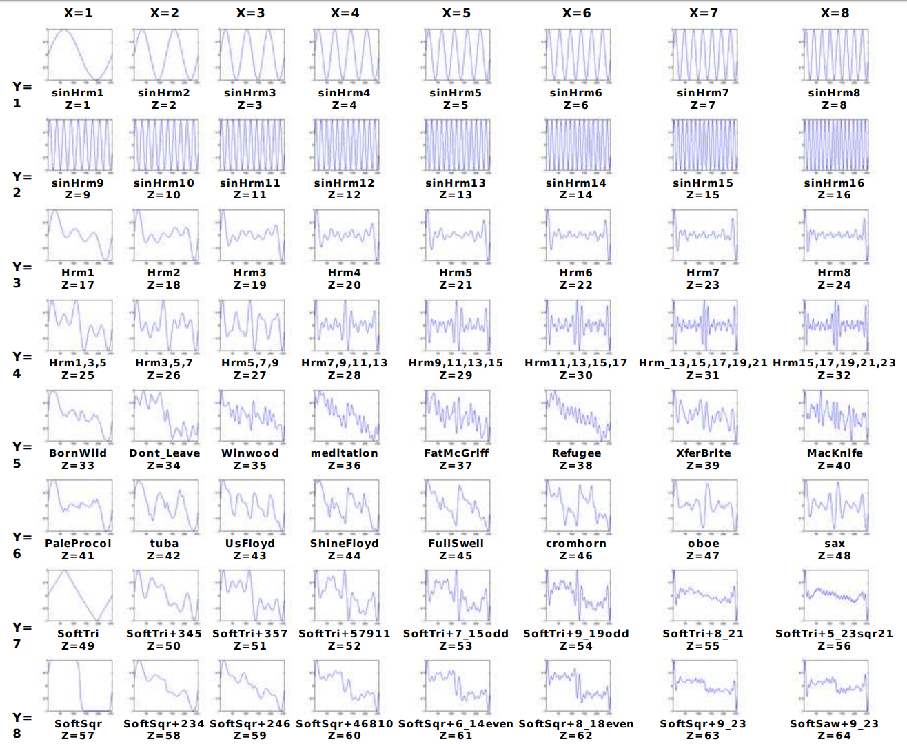
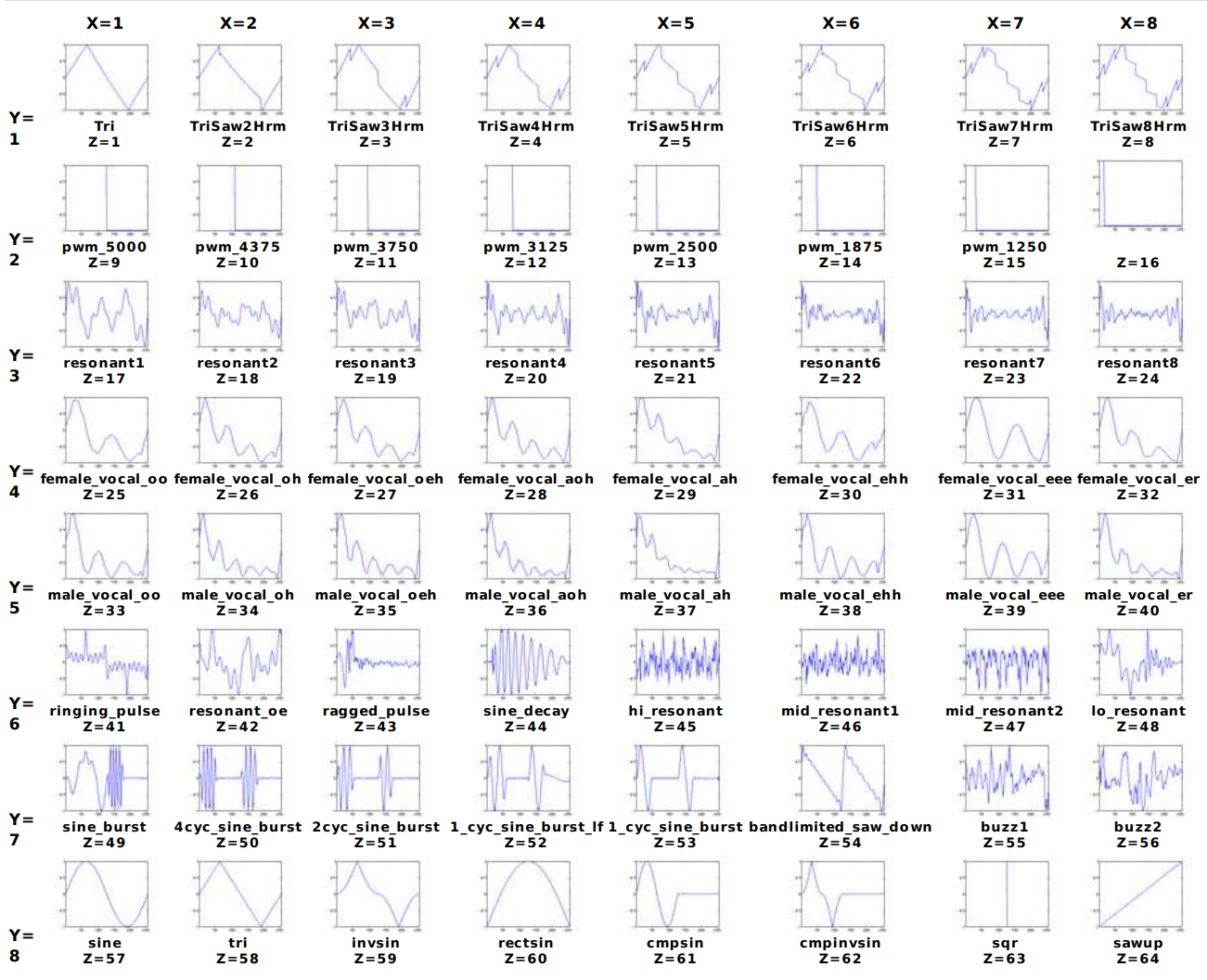
Each index of 64 waves was arranged as an 8x8 array. The “rows” are represented on the X axis and the “columns” on the Y axis (pictured above). The third array (Z index) adds depth to the X,Y array. In this étude this lookup table is modulated with various sources including curvilinear shapes and smoothed bipolar Brownian motion. As the modulation source indexes through the positions in the table a smoothing function for “frame interpolation” has been applied to the waves. This smoothing/anti-aliasing algorithm allows the two outputs to be a continuous blending of one wave to another. During these iterations the algorithms’ calculation adds an order of magnitude of “in-between” waveforms, so that the 192 waveforms are expanded to over 24,000 possible timbres. In these studies no filtration was applied to avoid masking the timbral shifting generating the rich partial series.
Anti-aliasing function for higher-order integrated wavetable synthesis:
1. Kth order integration with cascaded first-order integrators
2. Table look-up and interpolation
3. Kth order differentiation with cascaded first-order differentiators
K = order of integration
N = order of polynomial interpolator
1. Kth order integration with cascaded first-order integrators
2. Table look-up and interpolation
3. Kth order differentiation with cascaded first-order differentiators
K = order of integration
N = order of polynomial interpolator
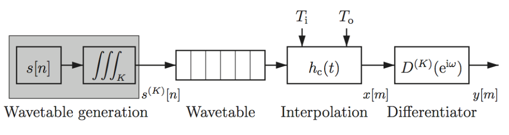
Franck & Välimäki 2013
- sine banks
- pulse width modulations
- filtered noise
- vocal formants
Spherical Vertex Interpolations
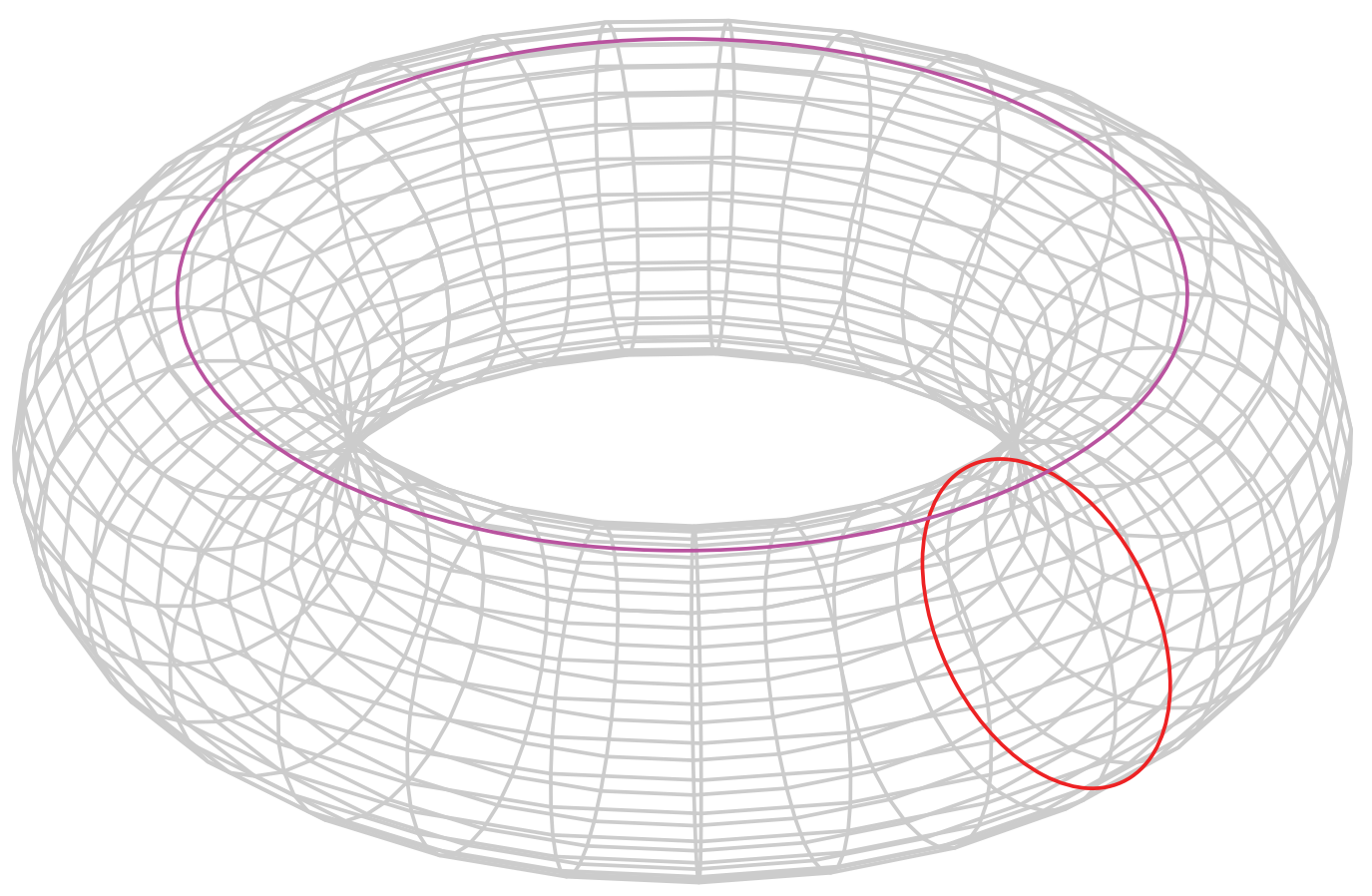
A spherical wavetable is another way of grouping waveforms. The modulation parameters for traversing the spherical wavetable in this study include latitude, longitude, and depth. The modulation index navigation morphs between waveforms positioned at various vertices on the surface of the geometry. Although the term “sphere” when talking about the wavetables, the structure of each wavetable is actually a 3-torus.
“What’s a 3-torus? A three-dimensional structure existing in a four-dimensional space. To understand what a 3-torus is, first think about a circle. A circle is a single dimensional object that wraps around to its beginning point as it reaches its end point. Any point on the circumference of a circle can be specified by a single number (by an angle from 0° to 360°), so a circle is one-dimensional. However, in order to draw a circle you need a two-dimensional space such as a piece of paper. So, a circle is a one-dimensional object existing in a two-dimensional space. Now, think about a doughnut (a torus, see picture below). You can make a donut if you extrude a circle into a cylinder and then bend the cylinder around so the top and bottom faces are touching. You can specify any point on the surface of the doughnut with just two numbers (an angle of the original circle and a position along the extruded cylinder), so the torus surface is two-dimensional and clearly exists in a threedimensional space. The next step is not as easy to visualize — imagine you took a donut and extruded it through a fourth dimension, and then connected the beginning to the end. This is a 3-torus. It’s a three-dimensional object that exists in a four-dimensional space. If you happened to be on the surface of a 3-torus and you looked far enough in any direction you’d see the back of your own head! If you walked far enough in any direction you’d end up exactly where you started, facing the same direction. The same is true for these wavetables: if you navigate far enough in any direction, you end up back to where you started.”
Stochastic Matrices & Steady State Transitions
In this next étude I make use of Markov (stochastic) matrices as a method of using probability to index through the wavetables outlined in the first section. The modulation source steps through the Markov process (pictured below) resampling at 1Hz. Using this sample rate conversion technique, arbitrary musical pitches were generated indexing through the set of wavetables: downsampling was used for raising the pitch and upsampling for lowering it.
For posterity, let’s look at the properties of the stochastic matrix:
- In a stochastic matrix, all entries are nonnegative, and each column sums to 1.
- The product of stochastic matrices is stochastic.
- In a Markov chain, elements move from one state to another with the same probabilities at each step in the process.
- The transition matrix for a Markov chain is a stochastic matrix whose (i, j) entry gives the probability that an element moves from the jth state to the ith state during the next step of the process.
- The probability vector after n steps of a Markov chain is Mnp, where p is the initial probability vector and M is the transition matrix.
- A limit vector for a Markov chain is always a fixed point (a vector x such that M x = x, if M is the transition matrix).
- A stochastic square matrix is regular if some positive power has all entries nonzero.
- If the transition matrix M for a Markov chain is regular, then the Markov chain has a unique limit vector (known as a steady-state vector), regardless of the values of the initial probability vector.
- If the transition matrix M for a Markov chain is regular, the positive powers of M approach a limit (matrix) all of whose columns equal the chain's steady-state vector.
